Sequential Verilog
In the last chapter we discussed the language features of Verilog to describe purely combinational logic… We did this starting with a simple seven-segment decoder (code and testbench), continuing with the ripple-carry-adder as a second example and ending with the latch trap we discussed. In this chapter we take the leap from purely combinational Verilog logic to sequential logic… This adds another set of language features we already had a peek at…
Example 1: D-Flipflop vs. latch
We started explaining the differences between D-Flipflops and latches in chapter 12.
 1
 2
 3
 4
 5
 6
 7
 8
 9
10
// D-flip-flop: takes over d only at the rising edge of clk
module d_ff (
    input  wire clk,
    input  wire d,
    output reg  q
);
    always @(posedge clk) begin
        q <= d;
    end
endmodule
The difference between a D-Flipflop and a latch is that a D-Flipflop is edge-triggered (meaning it changes its output value only on positive clock edges), while a latch is level-triggered, meaning its output value changes every time, as long as the en(able) input is active.
 1
 2
 3
 4
 5
 6
 7
 8
 9
10
11
// D-latch: transparent while en = 1, holds its value while en = 0
module d_latch (
    input  wire en,
    input  wire d,
    output reg  q
);
    always @(*) begin
        if (en)
            q <= d;
    end
endmodule
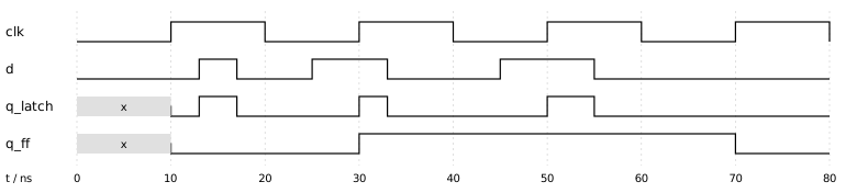
As can be seen in line 9 of the testbench shown below, the en(able) input is connected to the clock of the testbench, while for the D-flipflop the clock also goes into the clock input. Thus, both the flipflop and the latch receive the same signals, but react to different time spans: the latch reacts during the whole time frame, while the flipflop only changes on edges…
Inputs never change on edges.
This has two reasons. In real hardware, the input of a flipflop must be stable shortly before and after the edge (setup and hold times; see chapter 22). If it changes exactly at the edge, the result is unpredictable. In a simulation, the result would be ambiguous as well: if two events occur at the same time, the result depends on the order in which the simulator processes them. This is called a race condition.
 1
 2
 3
 4
 5
 6
 7
 8
 9
10
11
12
13
14
15
16
17
18
19
20
21
22
23
24
25
26
27
28
29
30
31
`timescale 1ns / 1ps

module latch_vs_ff_tb;
    reg  clk = 0;
    reg  d   = 0;
    wire q_latch, q_ff;

    // the clock is used as enable for the latch
    d_latch latch (.en(clk), .d(d), .q(q_latch));
    d_ff    ff    (.clk(clk), .d(d), .q(q_ff));

    // clock: period 20 ns
    always #10 clk = ~clk;

    initial begin
        $dumpfile("latch_vs_ff.vcd");
        $dumpvars(0, latch_vs_ff_tb);

        #13 d = 1;    // clk = 1: latch follows, flip-flop holds
        #4  d = 0;    // clk = 1: latch follows
        #8  d = 1;    // clk = 0: both hold, both take 1 at the edge at 30 ns
        #8  d = 0;    // clk = 1: latch follows, flip-flop holds
        #12 d = 1;    // clk = 0: both hold, both take 1 at the edge at 50 ns
        #10 d = 0;    // clk = 1: latch follows, flip-flop holds
        #25;
        $finish;
    end

    initial
        $monitor("t=%0d ns  clk=%b d=%b  q_latch=%b q_ff=%b", $time, clk, d, q_latch, q_ff);
endmodule
$monitor: This system function is called once and then remains active. As soon as one of the listed signals changes, it outputs a line—at most one per time step. That is why the lines shown above appear. Unlike $display, which outputs exactly once when it is called, $monitor monitors continuously.
The waveform
Next, we have a look at the waveforms. The clock is high from 10-20ns, 30-40ns, 50-60ns and finally 70-80ns. During these times the latch is open.
Initially, both outputs (the one from the latch and the flipflop) are in the state x, meaning unknown…
The latch only gets a value when it opens at 10 ns; the flipflop takes the value on the positive edge, also at 10 ns. After that, both are zero.
In summary: The flip-flop checks only four times—at 10, 30, 50, and 70 ns—and holds the value in between. The latch monitors the signal the entire time the clock is at 1.
Example 2: Shift register
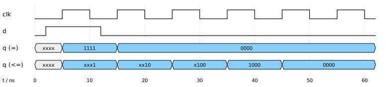
Both of the following Verilog sources should describe the same hardware, a 4-bit shift register, but there is a trap:
The reason is that the assignment syntax "=" does not work but must be replaced by "⇐"; you can ask an LLM of your choice for the concrete reasons.
The first one shows a non-blocking shift register - the one we want to have most of the time, while the second version is blocking…
 1
 2
 3
 4
 5
 6
 7
 8
 9
10
11
12
13
// RIGHT: non-blocking assignments (<=) in a clocked block
module shift_reg (
    input  wire       clk,
    input  wire       d,
    output reg  [3:0] q
);
    always @(posedge clk) begin
        q[0] <= d;
        q[1] <= q[0];
        q[2] <= q[1];
        q[3] <= q[2];
    end
endmodule
 1
 2
 3
 4
 5
 6
 7
 8
 9
10
11
12
13
// WRONG: blocking assignments (=) in a clocked block
module shift_reg_blocking (
    input  wire       clk,
    input  wire       d,
    output reg  [3:0] q
);
    always @(posedge clk) begin
        q[0] = d;
        q[1] = q[0];
        q[2] = q[1];
        q[3] = q[2];
    end
endmodule
As the waveform of the testbench shows, the results of the first and the second version are quite different…
 1
 2
 3
 4
 5
 6
 7
 8
 9
10
11
12
13
14
15
16
17
18
19
20
21
22
23
24
25
26
27
28
`timescale 1ns / 1ps

module shift_reg_tb;
    reg        clk = 0;
    reg        d   = 0;
    wire [3:0] q_blocking, q_nonblocking;

    shift_reg_blocking bad  (.clk(clk), .d(d), .q(q_blocking));
    shift_reg          good (.clk(clk), .d(d), .q(q_nonblocking));

    // clock: period 10 ns
    always #5 clk = ~clk;

    initial begin
        $dumpfile("shift_reg.vcd");
        $dumpvars(0, shift_reg_tb);

        // shift in the pattern 1, 0, 0, 0, 0, ...
        #2  d = 1;
        #10 d = 0;
        #50;
        $finish;
    end

    // print both registers after every rising clock edge
    always @(posedge clk)
        $strobe("t=%0d ns  d=%b  blocking q=%b  non-blocking q=%b", $time, d, q_blocking, q_nonblocking);
endmodule
Example 3: A counter
 1
 2
 3
 4
 5
 6
 7
 8
 9
10
11
12
13
14
15
16
17
18
19
20
21
22
// up/down counter from 0 to MOD-1 with synchronous reset and enable
module counter_updown #(
    parameter WIDTH = 4,
    parameter MOD   = 10
) (
    input  wire             clk,
    input  wire             rst,
    input  wire             en,
    input  wire             up,
    output reg  [WIDTH-1:0] q
);
    always @(posedge clk) begin
        if (rst)
            q <= 0;
        else if (en) begin
            if (up)
                q <= (q == MOD - 1) ? 0 : q + 1;
            else
                q <= (q == 0) ? MOD - 1 : q - 1;
        end
    end
endmodule
Introducing Parameters
As you can see above, this time we introduce parameters to the code:
First we handle the bit width WIDTH, second the modulo counter MOD.
This parameterisation eases the implementation of fine-tunable circuits. We know the bit width from the example with the ripple-carry adder.
The modulo-10 counter, for example, is used in the 7-segment display.
Priority of conditions
The reset "if (rst)" is checked first, so it always takes effect, no matter whether en is 0 or 1. Only after that comes "else if (en)": without enable, the counter simply holds its value. Since this happens in a clocked block, no latch is created, but a flipflop that keeps its value.
Synchronous Reset
Because the reset sits inside the "always @(posedge clk)" block, it only takes effect on a clock edge. This is called a synchronous reset. The alternative is an asynchronous reset, which takes effect immediately, independent of the clock: "always @(posedge clk or posedge rst)".
The conditional operator
The expression "(q == MOD - 1) ? 0 : q + 1" reads like in the programming language C: when the counter is at 9, it becomes 0, otherwise it is incremented by one. Counting down works the same way: if the counter is 0, it becomes 9, otherwise it is decremented by one. In hardware, "? :" becomes a multiplexer; for this counter, Yosys creates 6 $MUX cells.
Overflow in both directions
The counter from chapter 22 overflows from 15 to 0, as it cannot hold more than 4 bits. Here, the overflow from 9 to 0 and from 0 to 9 is described explicitly.
What happens for the values 10 to 15?
After a reset, they never occur. Should the counter miscount into such a value, it recovers by itself: Upwards it goes from 12 to 13,14,15 back to zero, downwards it goes from 11 and 10 to 9. This is exactly the "pitfall of unused states" described in chapter 14, here solved (but only for real hardware, after 1 to 6 clock cycles).
The testbench
 1
 2
 3
 4
 5
 6
 7
 8
 9
10
11
12
13
14
15
16
17
18
19
20
21
22
23
24
25
26
27
28
29
30
`timescale 1ns / 1ps

module counter_updown_tb;
    reg        clk = 0;
    reg        rst = 1;
    reg        en  = 0;
    reg        up  = 1;
    wire [3:0] q;

    counter_updown #(.WIDTH(4), .MOD(10)) dut (
        .clk(clk), .rst(rst), .en(en), .up(up), .q(q)
    );

    // clock: period 10 ns
    always #5 clk = ~clk;

    initial begin
        $dumpfile("counter_updown.vcd");
        $dumpvars(0, counter_updown_tb);

        #12  rst = 0;
        #10  en  = 1;     // count up: 0 ... 9, 0 ... 3
        #130 up  = 0;     // count down: 2, 1, 0, 9, 8, 7
        #60;
        $finish;
    end

    always @(posedge clk)
        $strobe("t=%0d ns  rst=%b en=%b up=%b  q=%0d", $time, rst, en, up, q);
endmodule
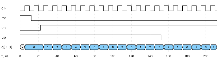
When the counter is instantiated with #(.WIDTH(4), .MOD(10)), the parameters are overridden: this is how a parameterised module is configured when it is embedded. The clock has a period of 10 ns, so the rising edges occur at 5, 15, 25 … ns. The stimuli follow one another with relative # delays: the reset ends at 12 ns, en goes to 1 at 22 ns, up goes to 0 at 152 ns, and the simulation ends at 212 ns. Because $strobe sits in an "always @(posedge clk)" block, it prints one line per rising edge, with the value that has settled at the end of that time step.
In the waveform, q is unknown (x) for the first 5 ns, until the first edge with active reset sets it to 0. Without a reset, the simulation would stay at x forever: x + 1 is x again, and so is the comparison with 9. From 25 ns on, the counter counts up from 1 to 9, wraps from 9 to 0 at 115 ns and continues to 3. From 155 ns on it counts down, wraps from 0 to 9 at 185 ns and ends at 7. Only the values 0 to 9 ever appear.
Synchronous instead of asynchronous
The binary counter from chapter 12 was asynchronous: Every Flipflop was clocked by the output of the previous stage. Here, all Flipflops are connected to the same clock, so they switch concurrently. This is the way counters in modern circuits are wired.
What Yosys synthesizes
33 cells, including 4 × $SDFFE_PP0P: Those are flipflops with internal synchronous reset and enable. So Yosys recognizes the structure "if (rst) … else if (en)" and generates the appropriate Flipflops. The remaining cells are used by the increment and decrement logic, the comparison and the selection.
Example 4: A traffic light
Let’s build the traffic light example from chapter 14 into a concrete description of the schematic based on Verilog.
The traffic light is the Moore automaton from chapter 14: four states (red, red-yellow, green, yellow), binary coded as 00, 01, 10, 11, and all three outputs depend only on the state. In chapter 14 we derived the boolean equations by hand: Q0' = ¬Q0, Q1' = Q1 ⊕ Q0, R = ¬Q1, Y = Q0, G = Q1 · ¬Q0. The result was "two D-flipflops, two inverters, one XOR gate and one AND gate". Yosys confirms this: traffic_light_eq.v is synthesized to 2 flipflops, 2 inverters, 1 XOR and 1 ANDNOT (an AND with one inverted input).
 1
 2
 3
 4
 5
 6
 7
 8
 9
10
11
12
13
14
15
16
17
18
19
20
21
22
23
24
25
26
27
// traffic_light_eq.v
// traffic light as Moore machine, built from the equations of chapter 14
// next state:  Q0' = ~Q0,  Q1' = Q1 ^ Q0
// outputs:     R = ~Q1,  Y = Q0,  G = Q1 & ~Q0
module traffic_light_eq (
    input  wire clk,
    input  wire rst,
    output wire r,
    output wire y,
    output wire g
);
    reg q1, q0;

    always @(posedge clk) begin
        if (rst) begin
            q1 <= 1'b0;
            q0 <= 1'b0;
        end else begin
            q0 <= ~q0;
            q1 <= q1 ^ q0;
        end
    end

    assign r = ~q1;
    assign y = q0;
    assign g = q1 & ~q0;
endmodule
Two different models
The traffic_light_eq.v above writes the equations directly in Verilog. The two flipflops q1 and q0 sit in a clocked block with ⇐, and the outputs are three assign statements, exactly the boolean equations from chapter 14. This is compact, but you have to derive the boolean equations yourself, and for big automata this quickly becomes confusing.
 1
 2
 3
 4
 5
 6
 7
 8
 9
10
11
12
13
14
15
16
17
18
19
20
21
22
23
24
25
26
27
28
29
30
31
32
33
34
35
36
37
38
39
40
41
42
43
44
45
46
47
// traffic_light.v
// traffic light as Moore machine with named states
module traffic_light (
    input  wire clk,
    input  wire rst,
    output reg  r,
    output reg  y,
    output reg  g
);
    localparam RED        = 2'b00;
    localparam RED_YELLOW = 2'b01;
    localparam GREEN      = 2'b10;
    localparam YELLOW     = 2'b11;

    reg [1:0] state, next;

    // state register
    always @(posedge clk) begin
        if (rst)
            state <= RED;
        else
            state <= next;
    end

    // next-state logic
    always @(*) begin
        case (state)
            RED:        next = RED_YELLOW;
            RED_YELLOW: next = GREEN;
            GREEN:      next = YELLOW;
            YELLOW:     next = RED;
            default:    next = RED;
        endcase
    end

    // output logic: depends only on the state (Moore)
    always @(*) begin
        {r, y, g} = 3'b000;
        case (state)
            RED:        {r, y, g} = 3'b100;
            RED_YELLOW: {r, y, g} = 3'b110;
            GREEN:      {r, y, g} = 3'b001;
            YELLOW:     {r, y, g} = 3'b010;
            default:    {r, y, g} = 3'b100;
        endcase
    end
endmodule
traffic_light.v: The common style with named states
Here, localparam gives names to the states: RED, RED_YELLOW, GREEN and YELLOW. In contrast to a normal parameter, a localparam is only valid inside its module and cannot be overridden from outside.
The module consists of three blocks, and they correspond exactly to the blocks of the block diagram from chapter 14. The state register is an "always @(posedge clk)" block with ⇐, the blue block in the diagram. The transition logic δ is an "always @()" block with a case statement that computes next from state. The output logic λ is another "always @()" block with case that computes R, Y and G from state alone, which makes it a Moore automaton. This is the rule of thumb from the shift register in its purest form: ⇐ in clocked blocks, = in combinational blocks.
The big advantage: there are no boolean equations to derive. The automaton is described just like in the state diagram, and the synthesis tool derives the equations itself.
Testbench and Waveform
 1
 2
 3
 4
 5
 6
 7
 8
 9
10
11
12
13
14
15
16
17
18
19
20
21
22
23
24
25
26
27
28
29
30
31
32
33
`timescale 1ns / 1ps

module traffic_light_tb;
    reg  clk = 0;
    reg  rst = 1;
    wire r_eq, y_eq, g_eq;
    wire r, y, g;
    integer errors = 0;

    traffic_light_eq by_hand (.clk(clk), .rst(rst), .r(r_eq), .y(y_eq), .g(g_eq));
    traffic_light    named   (.clk(clk), .rst(rst), .r(r),    .y(y),    .g(g));

    // clock: period 10 ns
    always #5 clk = ~clk;

    initial begin
        $dumpfile("traffic_light.vcd");
        $dumpvars(0, traffic_light_tb);
        #12 rst = 0;
        #100;
        if (errors == 0) $display("PASSED: both implementations are identical");
        else             $display("FAILED: %0d differences", errors);
        $finish;
    end

    // compare both implementations after every rising clock edge
    always @(posedge clk) begin
        #1;
        $display("t=%0d ns  state=%b  R=%b Y=%b G=%b", $time, named.state, r, y, g);
        if ({r_eq, y_eq, g_eq} !== {r, y, g})
            errors = errors + 1;
    end
endmodule
The Testbench
This testbench works differently from the previous ones: It not only stimulates a circuit, but also compares two
implementations with each other. To do this, both modules are instantiated side by side. by_hand is traffic_light_eq.v with the
equations from Chapter 14, and named is traffic_light.v with the named states. Both receive the same clk and rst signals,
and their outputs are connected to separate lines. Apart from clk and rst, the traffic light has no inputs, so there is nothing else
to trigger: The reset ends at 12 ns, after which the automaton continues running on its own driven by the clock.
The comparison is performed after every rising edge, but only after #1. By that point, the non-blocking assignments have been processed in both modules. A comparison exactly on the edge would again result in a race condition, as we saw in Example 1. Using {r_eq, y_eq, g_eq}, the three outputs are combined into a 3-bit value, allowing them to be compared in a single step.
For the comparison, we use !== instead of !=. The difference lies in how x is handled: !== performs an exact comparison, including x. If one implementation returns x and the other returns a valid value, this counts as an error. With !=, the result would be x itself, and the if statement wouldn’t even be triggered.
For the output, the testbench uses named.state to access the internal state of the instance named, even though state is not a port at all. Such a hierarchical name only works in simulation. At the end, there is no longer a view of the output, but rather a verdict: PASSED or FAILED, along with the number of discrepancies.
Note: The testbench only checks whether both implementations output the same value; it does not check whether the output is valid. Without a reset, both remain at x the entire time, and for !==, x equals x. The testbench still reports PASSED.
The Waveform
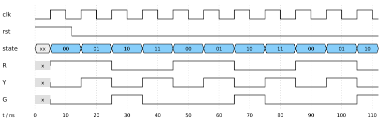
The waveform shows clk, rst, and state, as well as the outputs R (Red), Y (Yellow), and G (Green) of the named instance.
In the first 5 ns, state is still xx, and R, Y, and G are also unknown. Before the first edge, the flip-flops still
have no value, just like with the counter. The first rising edge at 5 ns occurs while reset is active and sets state to 00,
i.e., red. At 12 ns, rst goes low, and starting with the next edge at 15 ns, the state changes with each clock cycle—that is, every 10 ns:
from red (00) to red-yellow (01) and green (10) to yellow (11) and back to red. By the end of the simulation
at 112 ns, this cycle runs through just under three times.
It is notable that R, Y, and G change only in conjunction with state, that is, only at the edges. This is a hallmark of the
Moore automaton: The outputs depend exclusively on the state and not directly on an input. The values also match
the equations from Chapter 14. R = ¬Q1 is set in states 00 and 01, Y = Q0 in 01 and 11, and G = Q1 · ¬Q0 only in 10.
However, this is not yet a real traffic light, because each phase lasts exactly one clock cycle here. For phases of varying lengths, you would also need a counter that waits for a specific amount of time in each state.
One-hot: What Yosys Does with traffic_light.v
If you synthesize traffic_light.v with Yosys, the resulting circuit is not the one from Chapter 14. Yosys recognizes the state machine and re-encodes it using what’s known as one-hot encoding. In this process, each state gets its own flip-flop, and exactly one of them is set at any given time: 00 becomes 0001, 10 becomes 0010, 01 becomes 0100, and 11 becomes 1000.
The result is 13 cells, including 4 flip-flops instead of 2. By comparison, traffic_light_eq.v requires only 6 cells.
Using synth -nofsm disables the recoding; Yosys then retains the binary encoding and ends up with 11 cells
and 2 flip-flops.
Why does Yosys do this? Although one-hot encoding requires more flip-flops, the logic for each individual state is simpler and therefore faster. On FPGAs, which have many flip-flops anyway, this is often the better choice; more on this in Chapter 27. It’s important to note that the encoding is not specified in the Verilog code. The code describes the behavior; the encoding is chosen by the synthesis tool.
(Created with Claude AI)