Combinational Logic in Verilog
In the last chapter we already described a combinational circuit in Verilog:
the full adder, with two assign statements. For a single full adder that is enough.
For bigger circuits we need a few more tools: multi-bit signals, a way to describe a truth table
in a readable form, and a way to build big circuits from small ones.
In this chapter we learn these tools with two new circuits: a 7-segment decoder, which turns a number into the pattern for a digit display, and a ripple-carry adder, which we build from our full adders. At the end we look at the most common mistake when describing combinational logic.
Vectors and numbers
So far all our signals were a single bit. In Verilog, a signal can also be a vector of several bits:
1
2
wire [3:0] value;   // 4 bits: value[3] (MSB) ... value[0] (LSB)
wire [6:0] seg;     // 7 bits
The most important operations on vectors:
Notation | Meaning | Example |
| a single bit (bit select) | the third bit from the right |
| several bits (part select) | the two upper bits |
| concatenation - puts signals side by side |
|
| replication | the bit x four times |
Numbers are written with their width and base: 4’hA is the 4-bit number A (hexadecimal, i.e. 10),
7’b0111111 is a 7-bit binary number and 8’d200 is the decimal number 200 with 8 bits.
Writing the width explicitly avoids surprises - Verilog quietly cuts off or extends numbers of the wrong width.
Two ways to describe combinational logic
We already know the first way: a continuous assignment with assign. It describes a wire that is permanently
connected to the result of an expression - exactly like a gate whose output always follows its inputs.
The second way is an always block:
1
2
3
always @(*) begin
    // statements
end
The @() means: execute the block again whenever *any of the signals read in it changes.
The block therefore behaves like combinational logic as well. Inside it, we may use if, case and other statements,
which makes complex logic much more readable than one long boolean expression.
One thing confuses almost every beginner: a signal that is assigned inside an always block must be declared as reg.
Despite the name, a reg is not automatically a register. In an always @(*) block it becomes ordinary
combinational logic - the name only means that the signal is assigned in a procedural block.
Example 1: A 7-segment decoder
A 7-segment display consists of seven bars, called a to g:
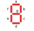
To show a digit, a specific combination of segments has to light up. For an 8 all seven are on, for a 1 only b and c. Our decoder receives a 4-bit number from 0 to F and outputs the seven segment signals. This is a combinational circuit with 4 inputs and 7 outputs - in other words, seven truth tables with 16 rows each.
With assign we would have to derive and simplify seven boolean equations. With a case statement we can write down
the truth table directly:
 1
 2
 3
 4
 5
 6
 7
 8
 9
10
11
12
13
14
15
16
17
18
19
20
21
22
23
24
25
26
27
28
// 7-segment decoder for the hexadecimal digits 0..F
// segment order: seg = {g, f, e, d, c, b, a}, 1 = segment on
module seven_seg (
    input  wire [3:0] value,
    output reg  [6:0] seg
);
    always @(*) begin
        case (value)
            4'h0: seg = 7'b0111111;
            4'h1: seg = 7'b0000110;
            4'h2: seg = 7'b1011011;
            4'h3: seg = 7'b1001111;
            4'h4: seg = 7'b1100110;
            4'h5: seg = 7'b1101101;
            4'h6: seg = 7'b1111101;
            4'h7: seg = 7'b0000111;
            4'h8: seg = 7'b1111111;
            4'h9: seg = 7'b1101111;
            4'hA: seg = 7'b1110111;
            4'hB: seg = 7'b1111100;
            4'hC: seg = 7'b0111001;
            4'hD: seg = 7'b1011110;
            4'hE: seg = 7'b1111001;
            4'hF: seg = 7'b1110001;
            default: seg = 7'b0000000;
        endcase
    end
endmodule
Every line of the case statement is one row of the truth table: for the input 4’h2, the segments g, e, d, b and a light up -
that is a 2. The bits of seg are ordered from g (bit 6) to a (bit 0).
Who turns this table into gates? The synthesis tool. It derives the boolean equations and simplifies them - exactly the work we did by hand with boolean algebra in part 1. For our decoder, the open-source synthesis tool Yosys generates about 30 gates.
Note | Many real displays are common anode: a segment lights up when its signal is 0, not 1.
For those displays, the output is simply inverted: assign seg_n = ~seg;. |
Testing the decoder
The testbench applies all 16 values one after another:
 1
 2
 3
 4
 5
 6
 7
 8
 9
10
11
12
13
14
15
16
17
18
19
20
`timescale 1ns / 1ps

module seven_seg_tb;
    reg  [3:0] value;
    wire [6:0] seg;
    integer i;

    seven_seg dut (.value(value), .seg(seg));

    initial begin
        $dumpfile("seven_seg.vcd");
        $dumpvars(0, seven_seg_tb);
        for (i = 0; i < 16; i = i + 1) begin
            value = i;
            #10;
            $display("value=%h  seg(gfedcba)=%b", value, seg);
        end
        $finish;
    end
endmodule
Instead of reading 16 rows of zeros and ones, we let a small script draw the segment patterns from the simulation output. This is the result of the simulation:

All 16 digits look right - including the lower-case b and d, which are needed so that they cannot be confused with 8 and 0.
Example 2: Hierarchy - a ripple-carry adder
Real designs are not one big module, but many small modules that are put together - just like in part 1, where we built an adder from full adders. In Verilog, we can use a module inside another module. This is called instantiation, and we already did it in the testbench of the last chapter.
A 4-bit adder consists of four full adders, where the carry output of each stage is connected to the carry input of the next stage:
 1
 2
 3
 4
 5
 6
 7
 8
 9
10
11
12
13
14
15
// 4-bit ripple-carry adder, built from four full adders
module ripple_adder4 (
    input  wire [3:0] a,
    input  wire [3:0] b,
    input  wire       cin,
    output wire [3:0] sum,
    output wire       cout
);
    wire [3:1] c;   // internal carries between the stages

    full_adder fa0 (.a(a[0]), .b(b[0]), .cin(cin),  .sum(sum[0]), .cout(c[1]));
    full_adder fa1 (.a(a[1]), .b(b[1]), .cin(c[1]), .sum(sum[1]), .cout(c[2]));
    full_adder fa2 (.a(a[2]), .b(b[2]), .cin(c[2]), .sum(sum[2]), .cout(c[3]));
    full_adder fa3 (.a(a[3]), .b(b[3]), .cin(c[3]), .sum(sum[3]), .cout(cout));
endmodule
Each line creates one full adder with its own name (fa0 to fa3). The internal wires c[1] to c[3] connect the carries.
Since the carry "ripples" from stage to stage, this circuit is called a ripple-carry adder.
Parameters and generate
For 4 bits, writing four lines is still fine. For 32 bits it would be tedious and error-prone. Verilog has two tools for this: a parameter makes the width configurable, and a generate loop creates the instances automatically:
 1
 2
 3
 4
 5
 6
 7
 8
 9
10
11
12
13
14
15
16
17
18
19
20
21
22
23
24
// N-bit ripple-carry adder, the full adders are generated in a loop
module ripple_adder #(
    parameter N = 8
) (
    input  wire [N-1:0] a,
    input  wire [N-1:0] b,
    input  wire         cin,
    output wire [N-1:0] sum,
    output wire         cout
);
    wire [N:0] c;   // c[0] = carry in, c[N] = carry out
    assign c[0] = cin;
    assign cout = c[N];

    genvar i;
    generate
        for (i = 0; i < N; i = i + 1) begin : stage
            full_adder fa (
                .a(a[i]), .b(b[i]), .cin(c[i]),
                .sum(sum[i]), .cout(c[i+1])
            );
        end
    endgenerate
endmodule
The for loop in the generate block is not executed at run time like a loop in software. It is expanded
before the simulation or synthesis: it simply produces N full adders, exactly as if we had written them by hand.
A 32-bit adder is now just ripple_adder #(.N(32)) add32 (…).
Testing the adder
For an 8-bit adder, we can still test all combinations - these are the \(2^{17} = 131072\) combinations
from the last chapter. The reference model is again simply the + operator:
 1
 2
 3
 4
 5
 6
 7
 8
 9
10
11
12
13
14
15
16
17
18
19
20
21
22
23
24
25
26
27
28
29
30
31
32
`timescale 1ns / 1ps

module ripple_adder_tb;
    localparam N = 8;

    reg  [N-1:0] a, b;
    reg          cin;
    wire [N-1:0] sum;
    wire         cout;
    integer i, j, k;
    integer errors = 0;

    ripple_adder #(.N(N)) dut (.a(a), .b(b), .cin(cin), .sum(sum), .cout(cout));

    initial begin
        // exhaustive test: 256 * 256 * 2 = 131072 combinations
        for (i = 0; i < (1 << N); i = i + 1)
            for (j = 0; j < (1 << N); j = j + 1)
                for (k = 0; k < 2; k = k + 1) begin
                    a = i; b = j; cin = k;
                    #1;
                    if ({cout, sum} !== a + b + cin) begin
                        if (errors < 10)
                            $display("ERROR: %0d + %0d + %0d = %0d", a, b, cin, {cout, sum});
                        errors = errors + 1;
                    end
                end
        if (errors == 0) $display("PASSED: all %0d combinations correct", (1 << (2*N)) * 2);
        else             $display("FAILED: %0d errors", errors);
        $finish;
    end
endmodule
The simulation takes less than a second:
PASSED: all 131072 combinations correct
By the way: in a real design you would simply write assign {cout, sum} = a + b + cin;. The synthesis tool
knows many adder structures and picks a suitable one. We build the adder ourselves here to practice hierarchy -
and because it shows what is behind the +. Its weakness is also visible: in the worst case the carry has to
ripple through all N stages, so the delay grows with the width. Faster adders, such as the carry-lookahead adder,
calculate the carries in parallel.
The classic pitfall: unintended latches
There is one mistake that almost everyone makes when starting with Verilog. Let’s look at a multiplexer that selects one of three 8-bit inputs:
 1
 2
 3
 4
 5
 6
 7
 8
 9
10
11
12
13
14
// WRONG: 3-to-1 multiplexer - the case for sel = 2'b11 is missing
module mux3 (
    input  wire [1:0] sel,
    input  wire [7:0] a, b, c,
    output reg  [7:0] y
);
    always @(*) begin
        case (sel)
            2'b00: y = a;
            2'b01: y = b;
            2'b10: y = c;
        endcase
    end
endmodule
The code compiles without errors. But sel has 2 bits and thus four possible values - and for 2’b11, no value is
assigned to y. What should the hardware do in this case? Verilog defines it: y keeps its old value.
Keeping a value means storing it - the combinational circuit has suddenly got a memory.
The simulation shows this clearly:

Between 20 and 40 ns, sel = 3. The output keeps the value 20 - even when input b changes to 99 at 30 ns.
A latch is a simple storage element that is controlled by the level of a signal, not by a clock edge: as long as it is enabled, its output follows the input, otherwise it holds its last value. The RS circuit from the chapter about clocks and flip-flops is such a latch. We will look at the difference between latches and flip-flops in detail in the next chapter.
The synthesis tool reacts in the same way: it builds a latch for every bit of y. Yosys reports this in its log:
Latch inferred for signal `\mux3.\y' ...
and the synthesized circuit contains 8 latches ($DLATCH_N), one per output bit.
That is a problem: latches are level-sensitive, can cause timing problems and are poorly supported on FPGAs -
and above all, nobody wanted them here.
The fix is simple: every output must get a value on every path through the always block.
Either with a default branch:
 1
 2
 3
 4
 5
 6
 7
 8
 9
10
11
12
13
14
15
// RIGHT: every path assigns a value to y
module mux3 (
    input  wire [1:0] sel,
    input  wire [7:0] a, b, c,
    output reg  [7:0] y
);
    always @(*) begin
        case (sel)
            2'b00:   y = a;
            2'b01:   y = b;
            2'b10:   y = c;
            default: y = 8'h00;
        endcase
    end
endmodule
or by assigning a default value at the beginning of the block, which is then overwritten where needed:
1
2
3
4
5
6
7
8
always @(*) begin
    y = 8'h00;           // default value
    case (sel)
        2'b00: y = a;
        2'b01: y = b;
        2'b10: y = c;
    endcase
end
With this, Yosys no longer generates any latches. This is also why our 7-segment decoder has a default branch,
although all 16 values are covered: it is a good habit that protects against this mistake.
The rules for combinational always blocks in short:
Use
always @(*), so that no input is forgotten.Assign a value to every output on every path - with
defaultor a default value at the beginning.Use the blocking assignment
=. (We will meet the non-blocking assignment<=in the next chapter, for flip-flops.)
Note | Try it yourself: with Yosys you can check any module for latches:
yosys -p "read_verilog mux3_latch.v; synth -top mux3; stat" prints the cells of the synthesized circuit.
If $DLATCH appears, a path is missing. |
Summary
Vectors, concatenation and sized numbers are the basic building blocks for multi-bit signals.
Combinational logic can be described with
assignor with analways @(*)block;casestatements describe truth tables directly.Modules can be instantiated inside other modules;
parameterandgeneratemake them configurable.An
always @(*)block in which an output is not assigned on every path creates an unintended latch.
In the next chapter we turn to sequential logic: flip-flops, registers, counters - and the traffic light from the chapter about finite state machines.
(Created with Claude AI)